FindMe Facial Recognition
Michael duPont
2017-04-18
Project Overview
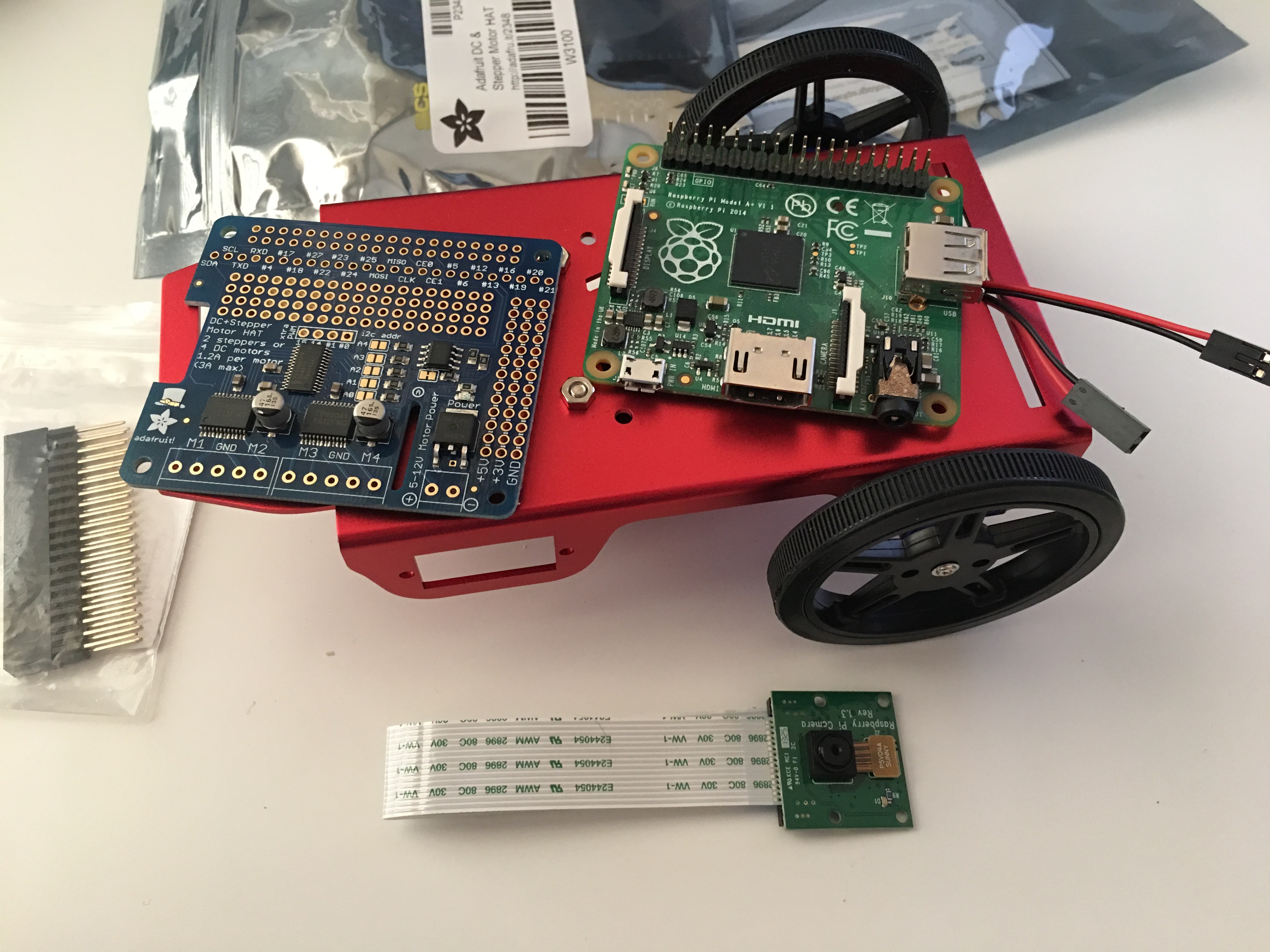
I am making a robot that can recognize and track me and only me. I'm building it using a Raspberry Pi running Raspbian, the official RPi camera module, a robot chasis and motor PHat from Adafruit, and Python to integrate the motors, camera, and facial recognition models. For the purposes of the capstone project, I will limit the scope of this report to the image processing and facial recognition portion of the overall project.
Problem Statement
Just focussing on the facial recognition component, we will need to train a model to find and recognize my face in an image. Those two verbs actually describe two different models we will need to have:
- Find - Locate all arbitrary faces in an image and return their locations
- Recognize - Determine if a given face is or is not the target face
There will need to be some handling between the two models, and we'll want all of this functionality wrapped into a single function. Here's what the image-model pipeline would look like:
- Function takes an image
- The first model finds all faces in the image and returns their bounding boxes
- Crop each face from its bounding box and scale to a standard size
- Feed each preprocessed face into the second model
- If the target face is found, return True and its bounding box
- If no faces are found or none of them belong to the target, return False and None
That should make the models easy to work with in the larger project code.
The first model will need to scan the image pixels looking for the best face candidates. Fortunately, this particular model is not project-specific, and I know where I can find and implement an existing one to save a lot of time. The second model will need to be trained to distinguish my face from others' given to it. I've implemented facial recognition using Scikit-Learn and SVMs before, but I want to use Keras (with TensorFlow) for this particular project. I've used it once before for object detection, and this seems like the perfect next step.
Metrics
Since we'll be making two separate models, we'll need two sets of metrics, but first here are some contextual definitions for each model that we'll use below:
- True Positive
- A bounding box containing a face
- A target face identified as the target
- False Positive
- A bounding box not containing a face
- A non-target face identified as the target
- True Negative
- A non-face not given a bounding box
- A non-target face not identified as the target
- False Negative
- A face not given a bounding box
- A target face not identified as the target
- Precision
- How many returned bounding boxes contain faces?
- How many of the faces identified as the target were actually the target?
- Recall
- How many faces in the image were given a bounding box?
- How many of the target faces were identified as the target?
Our first model needs to be able to identify all faces in an image while limiting the number of non-faces. We'll prioritize recall (how many ) for the first model since it's more important that every face be identified. Even if a few false positives make it to the second model, they should have little chance of passing a model trained to identify a specific face.
Because we're working with facial recognition, our second model needs to limit false positives more than True negatives. We'll prioritize precision for this second model because the model will constantly be fed images, and it is preferable for the model to be overly trained and miss a few valid frames.
Find Faces
The first thing we need to do is pick out faces from a larger image. Because the model for this is not user or case specific, we can use an existing model. Since we're going to be using OpenCV to do some image preprocessing, the easiest choice would be to use a Haar Cascade for finding each face. Briefly, a Haar Cascade is a series of hierarchical classifiers where the lowest levels look for specific orientations of points, edges, and lines. Check out OpenCV's documentation page on Haar Cascades for more info. There's a webpage I've used before which lists a few different Haar Cascades for body and face detection. This specific version will identify a full face when viewed from the front. We still have to tune a couple of hyperparameters, but it's better than having to build and train an entire model (which we will have to do later).
import cv2
import numpy as np

CASCADE = cv2.CascadeClassifier('findme/haar_cc_front_face.xml')

def find_faces(img: np.ndarray, sf=1.1282, mn=5) -> np.array([[int]]):
    """Returns a list of bounding boxes for every face found in an image"""
    return CASCADE.detectMultiScale(
        cv2.cvtColor(img, cv2.COLOR_RGB2GRAY),
        scaleFactor=sf,
        minNeighbors=mn,
        minSize=(30, 30),
        flags=cv2.CASCADE_SCALE_IMAGE
    )
That's really all we need. OpenCV has native support for cascade classifiers, which makes our model code short and simple. We have three tunable hyperparameters:
- Scale Factor: "How much the image size is reduced at each image scale." detectMultiScale will feed the given image into the cascade at different sizes to find the optimal bounding box. This affects the rate at which the image scales between runs.
- Minimum Neighbors: "How many neighbors each candidate rectangle should have to retain it." As the cascade builds up to larger candidate rectangles, the rectangle in the current layer must contain this minimum number of rectangles which passed the previous classifier.
- Minimum Size: "Minimum size of candidate rectangle" aka potential face. This will make the model a little faster and limit distant faces from being recognized.
Now let's test it by drawing rectangles around a few images of groups. Each individual is unique across every photo, which will be important in our next step. Here's one example:
import matplotlib.pyplot as plt
from matplotlib.image import imread, imsave
%matplotlib inline

plt.imshow(imread('test_imgs/initial/group0.jpg'))

from glob import glob

def draw_boxes(bboxes: [[int]], img: np.ndarray, line_width: int=2) -> np.ndarray:
    """Returns an image array with the bounding boxes drawn around potential faces"""
    for x, y, w, h in bboxes:
        cv2.rectangle(img, (x, y), (x+w, y+h), (0, 255, 0), line_width)
    return img

#Find faces for each test image
for fname in glob('test_imgs/initial/group*.jpg'):
    img = imread(fname)
    bboxes = find_faces(img)
    print('Bounding Boxes for file:', fname)
    print(bboxes, '\n')
    imsave(fname.replace('initial', 'find_faces'), draw_boxes(bboxes, img))

plt.imshow(imread('test_imgs/find_faces/group0.jpg'))

After tuning the hyperparameters, we're getting good face identification over our test images. We recognized all but two of the 29 faces in the images and had only one false positive pictured below. The two faces that it missed were tilted (one as much as 45°), and the model is only trained to find faces that are mostly upright (< 20°).
plt.imshow(imread('report_imgs/falsepositive.jpg'))

Now for this model's metrics. We said we'd focus on recall, but, while that is still true, we can't really measure it according to the definition. He's the problem with applying pure metrics in this case: there's no good way to get a meaningful value given that the number of true negatives vastly outnumbers true positives. There might only be a few faces in an image, but every attempted rectangle which is correctly identified as not a face is a true negative. Because of the way this classifier works, this leads to ratios like 100k false negatives and 2 true positives.
With that in mind, tuning the hyperparameters was more subjective than scientific, but I am confident that it is tuned well enough to compare to the benchmark.
Benchmark
Microsoft offers a similar service via its Azure Cognitive Services Face API. We'll use this as a benchmark tool for this part of the project. We'll use a client library to send our sample image to the service and draw the bounding boxes that it returns.
import cognitive_face as faceapi

faceapi.Key.set('ad4edd8c666e41638b199a3bb20c6216')


def bboxes_benchmark(img_path: str, display_path: str=None):
    """Displays an image with bounding boxes sourced by AzureCS Face API
    Can map the results onto a separate image if a display_path is given"""
    faces = faceapi.face.detect(img_path)
    bboxes = []
    for face in faces:
        rect = face['faceRectangle']
        bboxes.append([rect['left'], rect['top'], rect['width'], rect['height']])
    print(bboxes)
    plt.imshow(draw_boxes(bboxes, imread(display_path if display_path else img_path)))

bboxes_benchmark('test_imgs/initial/group0.jpg', 'test_imgs/find_faces/group0.jpg')

We're replicating what we just did, except we are now using a commercial service to return the bounding boxes instead of our model. In the test image, the green boxes were returned by our model, and the white boxes were returned by Face API. The commercial service was able to give a tighter bounding box for each face, but both versions were able to give roughly the same results and identify each face.
Build Dataset
Base Corpus
Now let's use this to build a base corpus of "these faces are not mine" so we can augment it later with the face we want to target. Because our first model feeds data into our second, it makes sense to use it to create our second model's training data. We'll use the faces from the test images in the previous section because all of them are unique and cover a decently wide demographic. The code below will use the bounding boxes to save cropped images of each found face.
#Creates cropped faces for imgs matching 'test_imgs/group*.jpg'

def crop(img: np.ndarray, x: int, y: int, width: int, height: int) -> np.ndarray:
    """Returns an image cropped to a given bounding box of top-left coords, width, and height"""
    return img[y:y+height, x:x+width]

def pull_faces(glob_in: str, path_out: str) -> int:
    """Pulls faces out of images found in glob_in and saves them as path_out
    Returns the total number of faces found
    """
    i = 0
    for fname in glob(glob_in):
        print(fname)
        img = imread(fname)
        bboxes = find_faces(img)
        for bbox in bboxes:
            cropped = crop(img, *bbox)
            imsave(path_out.format(i), cropped)
            i += 1
    return i

found = pull_faces('test_imgs/initial/group*.jpg', 'test_imgs/corpus/face{}.jpg')

print('Total number of base corpus faces found:', found)
plt.imshow(imread('test_imgs/corpus/face0.jpg'))

29 actual faces + 1 false positive - 2 false negatives = 28 corpus images
That verifies what we found earlier. I've manually removed the false positive pictured earlier from the corpus, so the final count comes to twenty-seven. Now that we have some faces to work with, let's save them to a pickle file for use later on.
from pickle import dump

#Creates base_corpus.pkl from face imgs in test_imgs/corpus
imgs = [imread(fname) for fname in glob('test_imgs/corpus/face*.jpg')]
dump(imgs, open('findme/base_corpus.pkl', 'wb'))
Target Corpus
Now we need to add our target data. Since this is going to power a personal project, I'm going to train it to recognize my face. Other than adding some new images, we can reuse the code from before but just supplying a different glob string.
found = pull_faces('test_imgs/initial/me*.jpg', 'test_imgs/corpus/me{}.jpg')

print('Total number of target faces found:', found)
plt.imshow(imread('test_imgs/corpus/me0.jpg'))

That was easy enough. In order to have a large enough corpus of target faces, I included pictures of myself with other people and deleted their faces after the code block ran. It ended up having thirteen target faces.
Model Training Data
Now that we have our faces, we need to create the features and labels that will be used to train our facial recognition model. We've already classified our data based on the face's filename; all we need to do is assign a 1 or 0 to each group for our labels. As for the images themselves, we'll need to scale each image to a standard size and remove the alpha channel (they're all 255). Thankfully the output for each bounding box is a square, so we don't have to worry about introducing distortions.
#Load the two sets of images
from pickle import load

notme = load(open('findme/base_corpus.pkl', 'rb'))
me = [imread(fname) for fname in glob('test_imgs/corpus/me*.jpg')]

print('Number of target faces:', len(me))
print('Number of non target faces', len(notme))

#Create features and labels
features = notme + me
labels = [0] * len(notme) + [1] * len(me)

#Preprocess images for the model
def preprocess(img: np.ndarray) -> np.ndarray:
    """Resizes a given image and remove alpha channel"""
    img = cv2.resize(img, (45, 45), interpolation=cv2.INTER_AREA)[:,:,:3]
    return img

features = [preprocess(face) for face in features]
Simple enough. Let's do a quick check before shuffling. The first image should be part of the base corpus:
print('Is the target:', labels[0] == 1)
plt.imshow(features[0], cmap='gray')

And the last image should be of the target:
print('Is the target:', labels[-1] == 1)
plt.imshow(features[-1], cmap='gray')

Looks good. Now that we have our full feature set, let's make two quick visualizations showing the entire corpus.
from matplotlib.gridspec import GridSpec

def make_grid(images: [np.ndarray], columns: int):
    """Displays an image grid for a given list of images"""
    rows = len(images) // columns + 1
    fig = plt.figure(figsize=(columns, rows))
    grid = GridSpec(rows, columns, wspace=0.0, hspace=0.0)
    for r in range(rows):
        for c in range(columns):
            image_index = r * columns + c
            if image_index >= len(images):
                break
            ax = plt.Subplot(fig, grid[r, c])
            ax.set_xticks([])
            ax.set_yticks([])
            ax.imshow(images[image_index], cmap='gray')
            fig.add_subplot(ax)
    plt.show()

print('Preprocessed Non-Target Faces Feature Set')
make_grid(features[:27], 6)

print('Preprocessed Target Faces Feature Set')
make_grid(features[-13:], 5)

Let's create a quick data and file checkpoint. This means we'll be able to load the file in from this point on without having to run most of the above code.
#Convert into numpy arrays
features = np.array(features)
labels = np.array(labels)

dump(features, open('test_imgs/features.pkl', 'wb'))
dump(labels, open('test_imgs/labels.pkl', 'wb'))
DATA/FILE CHECKPOINT
The report notebook can be run from scratch from this point onward. Note that the pkl files are not the same as above. This ensures that the model is trained on good data (ie false positives manually removed) and not accidentally overwritten.
from pickle import load
import numpy as np
import matplotlib.pyplot as plt
from matplotlib.image import imread, imsave
%matplotlib inline
from findme.imageutil import crop, draw_boxes, preprocess
from findme.models import find_faces

np.random.seed(42)

features = load(open('findme/features.pkl', 'rb'))
labels = load(open('findme/labels.pkl', 'rb'))

features = features[-26:]
labels = labels[-26:]
That's it for our data. You'll notice that we only loaded a subset of our dataset. We had 13 target faces, so we subset the last 13*2 faces from the feature set. This ensures that the number of target and non-target images matches, which leads to a better model even though it has less data overall. We'll split our data in the next section.
Am I in This?
We've already created all of our data. Now for the model we're going to train. First, we need to convert our labels to one-hot encoding for use in the model. This means our output layer will have two nodes: True and False.
from sklearn.preprocessing import OneHotEncoder

enc = OneHotEncoder()
labels = enc.fit_transform(labels.reshape(-1, 1)).toarray()
print('Not target label:', labels[0])
print('Is target label:', labels[-1])
Now we need to define our model architecture one layer at a time. We'll create three convolutional layers, two fully-connected layers, and the output layer.
from keras.layers import Activation, Convolution2D, Dense, Dropout, Flatten, MaxPooling2D
from keras.metrics import binary_accuracy
from keras.models import Sequential

SHAPE = features[0].shape
NB_FILTER = 16

def make_model() -> Sequential:
    """Create a Sequential Keras model to boolean classify faces"""
    model = Sequential()
    #First Convolution
    model.add(Convolution2D(NB_FILTER, (3, 3), input_shape=SHAPE))
    model.add(Activation('relu'))
    model.add(MaxPooling2D())
    model.add(Dropout(0.1))
    # Second Convolution
    model.add(Convolution2D(NB_FILTER*2, (2, 2)))
    model.add(Activation('relu'))
    model.add(MaxPooling2D())
    model.add(Dropout(0.2))
    # Third Convolution
    model.add(Convolution2D(NB_FILTER*4, (2, 2)))
    model.add(Activation('relu'))
    model.add(MaxPooling2D())
    model.add(Dropout(0.3))
    # Flatten for Fully Connected
    model.add(Flatten())
    # First Fully Connected
    model.add(Dense(1024))
    model.add(Activation('relu'))
    model.add(Dropout(0.4))
    # Second Fully Connected
    model.add(Dense(1024))
    model.add(Activation('relu'))
    model.add(Dropout(0.5))
    # Output
    model.add(Dense(2))
    model.compile(loss = 'mean_squared_error', optimizer = 'rmsprop', metrics=[binary_accuracy])
    return model

print(make_model().summary())
Now we need to train the model. Even though we have a large model in terms of its parameters, we can still let the model train for many epochs because our feature set is so small. On a MacBook Air, it takes around 30 seconds to train the model with 500 epochs. To save space, I've disabled the full training printout that Keras provides, but you can watch the accuracy progress yourself by changing verbose from 0 to 1.
We also need to shuffle our data because feeding all of the non-target and target faces into the model in order will lead to a biased model. Scikit-Learn has a convenient function to do this for us. Rather than just calling random, this function preserves the relationship between the feature and label indexes.
from keras.wrappers.scikit_learn import KerasClassifier
from sklearn.utils import shuffle

model = KerasClassifier(build_fn=make_model, epochs=500, batch_size=len(labels), verbose=0)
X, Y = shuffle(features, labels, random_state=42)
model.fit(X, Y)
Let's quickly see how well it trained to the given data. Because the dataset is so small, we didn't want to keep any for a test or validation set. We'll test it on a new image soon.
preds = model.predict(features)
print(preds[:13])
print('Non-target faces predicted correctly:', np.all(preds[:13] == 0))
print(preds[-13:])
print('Non-target faces predicted correctly:', np.all(preds[-13:] == 1))
That's it. This specific architecture started with LeNet and was customized through trial and error until the model performed well with the training set. Unlike the first model, this one was able to be evaluated objectively through its binary accuracy which you can view in the full training printout.
While Keras has its own mechanisms for training and validating models, we're using a wrapper around our Keras model so it conforms to the Scikit-Learn model API. We can use fit and predict when working with the model in our code, and it let's us train and use our model with the other helper modules sk-learn provides. For example, we could have evaluated the model using StratifiedKFold and cross_val_score which would look like this:
from keras.wrappers.scikit_learn import KerasClassifier
from sklearn.model_selection import StratifiedKFold, cross_val_score

model = KerasClassifier(build_fn=make_model, epochs=5, batch_size=len(labels), verbose=0)

# evaluate using 10-fold cross validation
kfold = StratifiedKFold(n_splits=3, shuffle=True, random_state=42)
result = cross_val_score(model, features, labels, cv=kfold)
print(result.mean())
This method allows us to determine how effective our model is but does not return a trained model for us to use.
Putting It Together
Lastly, let's create a single function that takes in an image and returns if the target was found and where.
First we'll load in our test image. Keep in mind that the model we just trained has never seen this image before and it contains multiple people (and a manatee statue).
test_img = imread('test_imgs/evaluate/me1.jpg')
plt.imshow(test_img)

Now for the function itself. Because we've already made functions around the core parts of our data pipeline, this final function is going to be incredibly short yet powerful.
def target_in_img(img: np.ndarray) -> (bool, np.array([int])):
    """Returns whether the target is in a given image and where"""
    for bbox in find_faces(img):
        face = preprocess(crop(img, *bbox))
        if model.predict(np.array([face])) == 1:
            return True, bbox
    return False, None
Yeah. That's it. Let's break down the steps:
find_facesreturns a list of bounding boxes containing faces- We prepare each face by cropping the image to the bounding box, scaling to 45x45, and removing the alpha channel
- The
modelpredicts whether the face is or is not the target - If the target is found (
pred == 1), return True and the current bounding box - If there aren't any faces or none of the faces belongs to the target, return False and None
Now let's test it. If it works properly, we should see a bounding bx appear around the target's face.
found, bbox = target_in_img(test_img)

print('Target face found in test image:', found)
if found:
    plt.imshow(draw_boxes([bbox], test_img, line_width=20))

Would you look at that. It works! We now have a single function to find and recognize my face in an arbitrary image just like we laid out at the beginning of this report.
Benchmark
Now it's time to benchmark this second model. We're again going to use Face API to identify the target face in an image. First we need to train the service to recognize the target face. We do this by creating a new person_id and upload each image to their cloud model. We then ask it to train our own model against a base corpus like we did in this project but on a much larger scale.
group_id = 0
faceapi.person_group.create(group_id, 'FindMe')
target_id = faceapi.person.create(0, 'Target')['personId']
print('Target ID:', target_id)

for face in glob('test_imgs/corpus/me*.jpg'):
    faceapi.person.add_face(face, group_id, target_id)

faceapi.person_group.train(group_id)
print('Target face trained in group', group_id)
Then we'll replicate target_in_image except using Face API for everything.
def target_in_image_faceapi(img_path: str, cutoff: float=0.66) -> (bool, np.array([int])):
    """Copy of target_in_image except built using Face API
    Returns True if target candidate confidence is above a given percentage"""
    faces = faceapi.face.detect(img_path)
    for i, person in enumerate(faceapi.face.identify([face['faceId'] for face in faces], group_id)):
        for candidate in person['candidates']:
            if candidate['personId'] == target_id and candidate['confidence'] >= cutoff:
                rect = faces[i]['faceRectangle']
                return True, [rect['left'], rect['top'], rect['width'], rect['height']]
    return False, None
Let's walk through this benchmark version:
detectreturns a list of faceIds and bounding boxesidentifyattempts to match each faceId to a personId in the trained groupId- We then look for any candidates matching in the group
- Returns True and the bounding box if both:
- A candidate's Id matches that of our target
- A candidate's confidence level is above a given threshold
- Returns False and None if no faces or candidates found
It's a little messier because we have to parse the returned JSON for each web call, but the heavy lifting is on the backend. One advantage this has over the other version is the ability to set the confidence level. This allows us to tune the sensitivity of the results. Now let's test it on the same image as before
found, bbox = target_in_image_faceapi('test_imgs/evaluate/me1.jpg')

print('Target face found in test image:', found)
if found:
    plt.imshow(draw_boxes([bbox], test_img, line_width=20))

There we go! Like we saw before, Face API gives the face a tighter bounding box, but we've verified the results of our facial recognition pipeline. In fact, our model was able to provide a more centered bounding box in this particular case. One downside to the Face API implementation is that the facial recognition is noticably slower because it's making multiple web calls to achieve the same effect. However, it might be necessary on devices which don't support or are not powerful enough to run a model on directly. Thankfully, this is not the case for the Raspberry Pi, and a local model would be preferable as speed is key to integrating it into a robotics project.
Results
When it comes to the two models, ours and the benchmark, the benchmark is far more robust given that it is trained over a larger dataset and we can tune the sensitivity. However, it is too slow for the robotics project since it will be reading images from the camera like a video stream. That's alright, though, because it performs well enough to miss a few frames. That is how we trained the model after all: recall for find and precision for recognize. We can trust our model when it says the target has been found while Face API is more likely to find it in more images.
Conclusion
Let's recap what we've done in this report. We started by implementing and tuning a Haar Cascade to find the best bounding box for every front-facing face in an image. We then used this first model to build our training set for our second model. We used a few photos to pull out 27 non-target faces and 13 target faces. Each cropped face was assigned a label and resized to 45x45x3 RGB pixels. We took a subset of our data so that our model would be trained on 13 faces of each type and converted the labels into one-hot encoding. The second model started as LeNet implemented with Keras and was customized to fit our use case. The model was trained quickly over 500 epochs with a small dataset but well enough to work with images it hasn't seen before. Finally we wrapped everything up into a single function that takes the raw image and outputs the is_found boolean and bounding box.
Even though I had implemented a Haar Cascade before, I was surprised how well this version worked before having to tune the hyperparameters. It took a little longer to tune it to get all of the upright faces without having too many false positives or drawing two different boxes around the same person.
The hardest part of the project was designing the second model's architecture. I lost so much time because I forgot to one-hot encode my labels. I kept getting very unreliable combinations of outputs because the output layer was only a single node. Once that was fixed, it was just a matter of increasing the epochs and a few more changes.
Improvements
The biggest limitation of this project is the dataset. I sourced all of the images of myself from my personal library, and I don't have a lot of unique photos of myself (not about that Instagram life). This meant that the training set was always going to be small, but we were still able to train the convnet to identify me in images it hadn't seen before.
It's possible that the second model won't work perfectly once it receives images from the robot via the RPi camera module. If this happens, I would augment and/or replace the image corpus with images taken by the camera module. However, this would have the opposite problem; I can take as many images of myself as I want, but my non-target corpus would be limited because I can't just start taking pictures of strangers with a battery-powered Raspberry Pi.